
Remote energy monitoring and optional control systems are designed for large facilities such as industrial factories, with some degree of automation.
Edge devices collect data from sensors, telemetry streams, user inputs or pre-programmed procedures and send it to CALMS cloud. The data it there stored, aggregated and analyzed. It can be then accessed via CALMS web application at app.calms.com.
Once limited to SCADA in industrial settings, remote monitoring and control is now applied in numerous fields, including energy systems:
- Compressed air
- Electricity
- Steam
- Air conditioning
- Gas
- Water
System
A system is a collection of elements or components that have common source of production, distribution and demad. E.g Company X can have two different systems, one Low pressure system and one High pressure system, with different supply, distribution network and demand (users).
Channels
Channel within CALMS platform represents an individual signal that we are observing. Channel is a entity that belongs to a Calms energy system and represents a measured or calculated signal.
- manual entries (adding and hiding data)
- pre-aggregation (fast querying of large periods)
Types
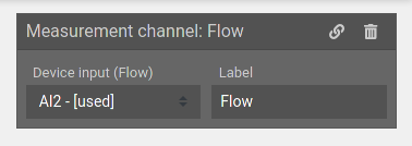
Measurement channel receives data from edge device’s inputs.
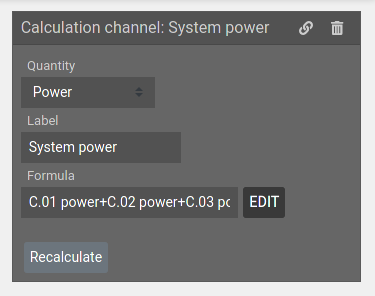
Calculation channel evaluates an expression (also known as formula) composed from mathematical functions, other channels and system variables (i.e. electricity cost).
Virtual channel is a channel that does not have a stored signal, but is calculated on-the-fly. This is necessary only because the value of this channel is dependent on the aggregation used, meaning that its values cannot be computed in advance.
It is specifically designed for SSP, which is defined as mean(POWER) / mean(FLOW).
It requires special treatment:
- it cannot display non-aggregated values
- it cannot use manual entries
- it cannot have alerts
Metric channel is a channel similar to measurement channel, but instead of receiving values from device inputs it receives them from various system metrics, for example waste flow, efficiency and reliability score.
This channel type cannot be implemented as a calculation channel, because calculation expression must contain at least one other channel. This is required since calculation channels are only recalculated on changes of that other channel. To work around this problem we could:
- evaluate and save the value of the system metric on every ingestion (very inefficient, these metrics will rarely change)
- just write the value into the channel when it changes, without triggering expression evaluation (this would actually become measurement channel - there is no point in pretending this is a calculation).
But it also cannot be measurement channel because it would be hard to enforce consistency with relations to device inputs and system metrics.
To see the list of channels in your system, visit system setup and select “Channels” tab.
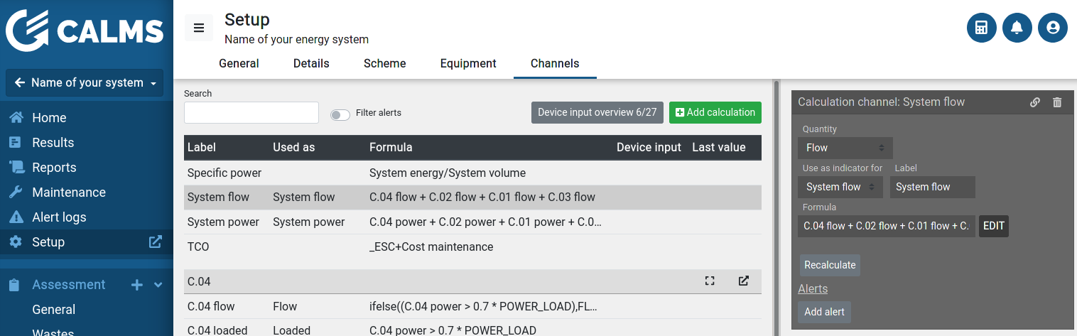
Channels can receive data from various sources:
Measurement channels read edge device inputs directly. Only configuration required is selection of the device input to be read from.
Calculation channels use a mathematical expression to compute value of the signal from other channels. Configuration requires the formula to be used and the quantity of result of the calculation.
Metric channels provide signals from other parts of CALMS platform such as Reliability and efficiency score from assessments.
Virtual channels are used in some specific cases to aggregate your data correctly. You will encounter them when configuring System Specific Power (SSP).
Units
CALMS is using all major units of measurement used for energy measurements, like flow, pressure, power, current, temperature, speed, frequency …
All channels in CALMS are stored in International system of units - SI units in database and can be converted any time to major or custom defined units by user.
Flow
CALMS Free air delivery (FAD or f.a.d) — the actual quantity of compressed air converted back to the inlet conditions of the compressor.
CALMS flow units should be measured or recalculated to Normal reference conditions: 101,3 kPa, 0°C (32°F), 0% RH.
Note: The units for FAD are cfm in the imperial system and m3/min or l/min in the metric system. The units are in general measured according to the ambient inlet standard conditions found in ISO 1217.
There is no universal standard for rating air compressors, air equipment and tools. Common terms are:
- CFM
- ICFM
- ACFM
- FAD
- ANR
- SCFM
- nl/min
CFM
- CFM (Cubic Feet per Minute) is the imperial method of describing the volume flow rate of compressed air. It must be defined further to take account of pressure, temperature and relative humidity - see below.
ICFM
- ICFM (Inlet CFM) rating is used to measure air flow in CFM (ft3/min) as it enters the air compressor intake .
ACFM
- ACFM (Actual CFM) rating is used to measure air flow in CFM at some reference point at local conditions. This is the actual volume flow rate in the pipework after the compressor.
FAD
- FAD (Free Air Delivery) (f.a.d) is the actual quantity of compressed air converted back to the inlet conditions of the compressor. The units for FAD are CFM in the imperial system and l/min in the SI system. The units are in general measured according the ambient inlet standard conditions ISO 1217: Ambient temperature = 20oC, Ambient pressure = 1 bar abs, Relative humidity = 0%, Cooling water/air = 20oC and Effective working pressure at discharge valve = 7 bar abs.
- 1 m3/min (f.a.d) = 1000 liter/min (f.a.d) = 1000 dm3/min (f.a.d) = 16.7 l/s (f.a.d) = 16.7 dm3/s (f.a.d) = 35.26 ft3/min (f.a.d) - please refer to CALMS Unit converter calculator.
ANR
- ANR (Atmosphere Normale de Reference) is quantity of air at conditions 1.01325 bar absolute, 20oC and 65% RH.
SCFM
- SCFM (Standard CFM) is the flow in CFM measured at some reference point but converted back to Standard Reference Atmosphere conditions 14.696 psia, 60oF.
nl/min
- nl/min is the flow in l/min measured at some reference point but converted to normal air conditions 1.01325 bar absolute, 0oC and 0% RH.
ISO 1217
- standard reference ambient conditions - temperature 20oC, pressure 1 bar abs, relative humidity 0%, cooling air/water 20oC, and working pressure at outlet 7 bar absolute.
The relation between the two volume rates of flow is (note that the simplified formula below does not account for humidity) - use CALMS calculator (Unit converter):
qFAD = qN * (TFAD/TN) * (PN/PFAD)
qFAD = qN * (273 + 20)/273 * (1.01325/1.00)
qFAD = qN * 1.0872
qFAD = Free Air Delivery (l/s)
qN = Normal volume rate of flow (Nl/s)
TFAD = standard inlet temperature (20°C)
TN = Normal reference temperature (0°C)
pFAD = standard inlet pressure (1.00 bar (abs.))
pN = Normal reference pressure (1.01325 bar(abs.))
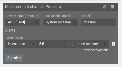
Alarms
Every channel (expect virtual ones) can be set to trigger an alarm in specific conditions. For example, when pressure falls below a specific value.
Key performance indicators
The easiest way to summarize performance of an energy system is to observe key performance indicators (KPI). CALMS web application shows then under Results page:
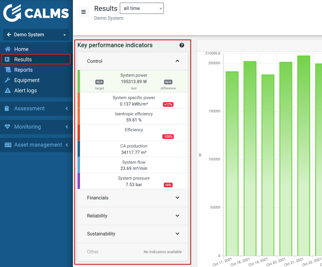
Indicator reference
System Specific Power and system specific energy
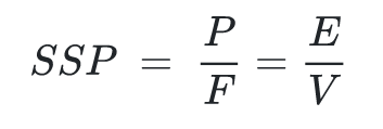
P … Power
F … Flow
E … Total electrical energy consumed
V … Total amount of air produced
System specific power is defined as average power divided by the average flow. This indicator is used to evaluate compressors. System specific energy is total energy used to produce a certain amount or volume of compressed air. This Indicator is an accurate way of determining the efficiency of a compressed air system.
SSP makes comparing compressors or compressor stations between themselves difficult because this indicator is sensitive to pressure. It can only be used to compare compressors or stations running at the same pressure. A compressor with lower efficiency may have a better (lower) specific power because it is compressing to a lower discharge pressure.
Isentropic Efficiency
As stated under System Specific Power SSP cannot be compared across systems operating at different pressures. A metric that can be used is isentropic efficiency. This metric incorporates the discharge pressure and can therefore be used to compare compressors or compressor stations of similar size even if they run at different operating pressures. Isentropic efficiency compares the actual energy consumption of a compressor or compressor station to the theoretical energy consumption of an idealized compressor. As this Idealized consumption cannot be realistically realized the actual number does not hold much meaning but is extremely useful when comparing several compressors or compressor stations between themselves.
To calculate the isentropic efficiency we can use this formula. All entries must be in primary ISO units
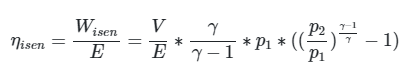
As “E/V” is actually SSP we can also write:
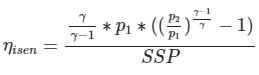
SSP in this case must be in Joules/cubic meter
p1 … input absolute pressure in Pascal (usually atmospheric pressure)
p2 … absolute discharge pressure in Pascal (atmospheric + gauge pressure)
V … volume of compressed air at inlet conditions (at input pressure and temperature (FAD)) in cubic meters
E … total energy used in Joules
γ … ratio of specific heats (assumed 1.4 for air)
Isentropic efficiency:
- < 50% - poor inefficient system
- 50-70% - average system efficiency
- 70-80% - good system efficiency
- 80-100% - very good system efficiency
- 100% - better then theoretically best system - system measurement or calculation error
100% measurement or calculation error
Usage of isentropic efficiency is considered more suitable for the following reasons:
Simplified comparison between different operating pressures / pressure ratios;
Isentropic efficiency is widely accepted in other (i.e. non-industrial air) technical fields like energy technology;
Isentropic efficiency is less sensitive regarding deviation of measurement conditions (operating point) and gas properties when comparing to specific power requirement;
Compressors without internal or interstage cooling are physically not able to compress isothermally;
Due to additional losses, even no compressor with internal cooling is able to reach even isentropic compression.
System redundancy
System redundancy or Available Redundant Capacity is the term used in capacity / power planning that customers may not know, but they do ask for it. What they ask is, “Can I safely add new compressed air user /line without overloading and potentially bringing down my facility? Or do I need to buy new compressor ?
Redundancy is a system design in which a biggest compressor is duplicated so if it fails there will be a backup. Redundancy has a negative connotation when the duplication is unnecessary or is simply the result of poor planning.
System redundancy = (Total system capacity - System flow capacity) / Biggest compressor capacity * 100%
System redundancy:
- < 100% - unreliable system without enough backup
- 100% - system has backup capacity for biggest compressor
- 100 - 200% - well designed and reliable system
- 200% - system with overcapacity
Some systems can have different redundancy requirements, like power plants they are aiming for 300%, pharmaceutical companies 200% …
Signals and summaries
This document explains how CALMS measures, transfers and aggregates signals - the underlying structure of channels.
Measurement
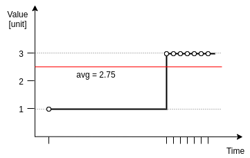
At first, we start with an analogue signal, that is being measured by the instruments.

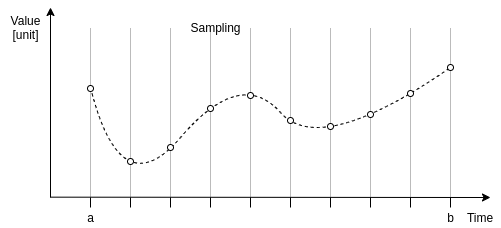
The result is so-called time-series: a series of data points of time and value.
To compute averages, integrals and other summaries, value of every point is extended up to the next data point measured. This behavior seems natural, because we can assume that the value of the signal is unchanged until we read a new value.
It is obvious that reconstructed signal is not equivalent to the original analog signal and that perfect fit would require infinite storage, bandwidth and computing power. To minimize the effective difference between the two while keeping relatively low size and complexity, we provide following settings:
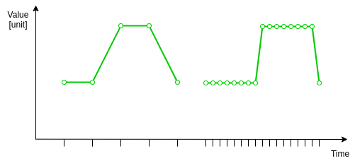
- Sampling interval can be configured separately for every device input. Usually, its value is set to 5 seconds. For signals that are known to change rapidly, it is recommended to be set this to 1 second.
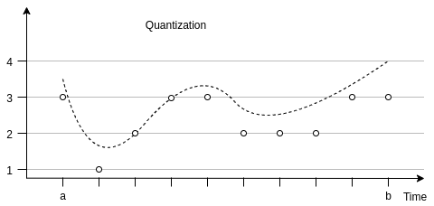
- Measurement precision represents minimal change required to
sample the signal. It can be utilized to significantly reduce
bandwidth usage. When:
- set to -1, the signal will be sampled regardless of the change
- set to 0, the signal will be sampled as soon as the value changes. This configuration does not have any effect on the resulting plots or statistics, but greatly reduces system load. Recommended for digital inputs, which were observed to reduce load by more than 90%.
- set to positive value, the signal will be sampled only when the value deviates from last value for more than this precision. It is recommended to match this setting with precision of your measurement equipment.
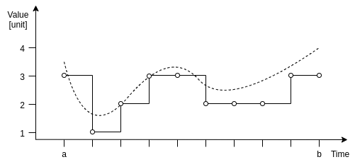
Alternative interpretations of the time-series as functions would include nearest neighbour and linear interpolation, but we have decided against these approaches due to significant increase of complexity they introduce. For more information, refer to the summaries section.
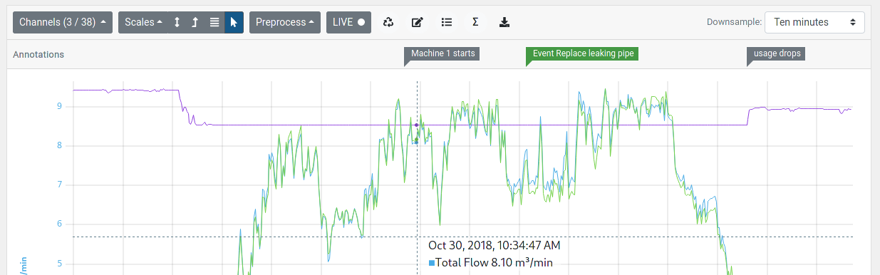
Plots
Plotting stepped signals is very inconvenient, because crossing lines may be hard to distinguish and look unnatural, especially with large time steps.
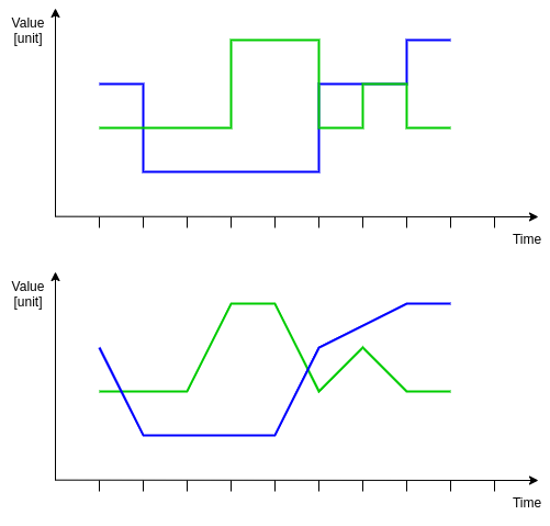
Instead, data points are linearly interpolated, resulting in more comprehensible plots.
It should be noted that when the plot is up-sampled (eg. as a result of plotting along signal with higher sample rate) it will increasingly start to look like the underlying stepped signal it represents.
Summaries
Even though the reconstructed signal is not equivalent to the original signal, it is used as its closest approximation and basis for all following processing. Because computational reproducibility is an important aspect of the monitoring pipeline, we will here explain how we calculate summaries in a way that can be reproduced in different parts of our application or by hand, to verify their integrity.
The two types of calculations we use are what we call aggregation and summary. Aggregation processes a signal and reduces its number of points, producing a new signal, while summary takes a signal and produces some statistic (eg. average).

Naive approach
The naive approach for both calculations (which we used for a long time) would be to use average of data point values. It turns out that this calculation is not stable and has many corner cases where it does not work. For example take a query of power usage for months of December, January and February with monthly aggregation:
| Period | Average of points | Pseudo-formula |
|---|---|---|
| December | 15kW | =AVG(Dec1 : Dec31) |
| January | 16kW | =AVG(Jan1 : Jan31) |
| February | 14kW | =AVG(Feb1 : Feb28) |
We can now compute summaries as average of averages:
| Total average power | 16kW | =(Dec+Jan+Feb) / 3 |
| Total energy used | 34560kWh | =TotalAvg * Duration(Dec:Feb) |
Unfortunately, both total power and energy used may be incorrect because:
Aggregation periods do not have equal duration. In this case, December and January have 31 days, while February has only 28 (or 29 depending on the leap year). To combat this, we should be calculating average, weighted with the period duration.
Some periods may contain missing data. In this case, December may have contained only 20 days of data, because the whole system (along with monitoring) was shut-down during the holidays.
Irregular sampling rate. When using precision on measurement inputs, sampled data points may not have uniform density, which breaks AVG operation.
Integral and duration
Instead of using average of data point values, we imitate weighted average by computing integral and duration of each data point. Duration is computed as time from current data point to the next one and the integral (of this square region) is just duration * value.
To compute weighted average of some period, we first sum all integrals, sum all durations and then divide the two.
| Period | Duration | Integral | Weighted average |
|---|---|---|---|
| Pseudo-formula | D | I | =I / D |
| December | 20 days | 7200 kWh | 15 kW |
| January | 31 days | 11904 kWh | 16 kW |
| February | 28 days | 9408 kWh | 14 kW |
| Total | 79 days | 28512 kWh | 15,038 kW |
| Pseudo-formula | =SUM(D) | =SUM(I) | =I / D |
In this way, we were able to construct an aggregation pipeline, that produces same results regardless the aggregation, missing data or irregular sampling rate.
Here is another example that demonstrates how this works on signals:
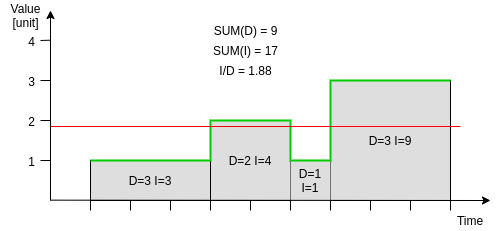
Notice how up-sampling of any of the chunks does not change the sums and the weighted average. If the second chunk (D=2 I=4) was split into two smaller chunks with (D=1 I=2), their total duration would still be 2 and integral would still be 4.
Warning about average of ratios
CALMS supports non-linear calculations (such as ratio), but it should be noted that their averages may not represent the result you intended to compute.
For example, take system specific power, ratio between power and flow.
| Period | Duration | Energy | Power | Volume | Flow | S. Spec. Power | Integral of SSP |
|---|---|---|---|---|---|---|---|
| Pseudo-formula | D | E | P=E/D | V | F=V/D | S=P/F | I=S*D |
| Thursday | 24 h | 360 kWh | 15 kW | 312 m3 | 13 m3/s | 1,15 kWs/m3 | 27,69 kWhs/m3 |
| Friday | 24 h | 384 kWh | 16 kW | 336 m3 | 14 m3/s | 1,14 kWs/m3 | 27,43 kWhs/m3 |
| Saturday | 24 h | 36 kWh | 1,5 kW | 9,84 m3 | 0,41 m3/s | 3,66 kWs/m3 | 87,80 kWhs/m3 |
| Total | 72 h | 780 kWh | 657,84 m3 |
Now, there are two approaches to calculating total system specific power:
- weighted average of SSPs of the periods (same as average of power or flow)
- using the formula on the totals (ratio between total avg. power and total avg. flow)
An honest mistake would be to use the first approach while the second is the one that you would usually want. It should be noted that they are not equivalent.
| Approach | Pseudo-formula | Result |
|---|---|---|
| 1.weighted average | =SUM(I) / SUM(D) | 1,99 kWs/m3 |
| 2.using totals | =[ SUM(E)/SUM(D) ] / [ SUM(V)/SUM(D) ] | 1,19 kWs/m3 |